Description of implementation approach and comments

從一般 BVH 架構中，一般都是用 full binary tree，子節點要不 0 個要不 2 個。若有 $N$ 個 primitive 物件，則表示有 $N$ 個葉節點放置這些 primitive 物件，而有 $N-1$ 個內部節點紀錄 Bounding Box 的部分。在測試交點和遍歷走訪的使用上，最慘有一半是多餘計算和走訪，而另一半屬於加速結構。

在論文 Ray Specialized Contraction on Bounding Volume Hierarchies 中，企圖想要利用 generic tree 取代一般使用 full binary tree 實作，在不更動 BVH 的效能下，減少運行上較沒用的內部節點，用以提升遍歷走訪效能，以及提升內存快取的效率。

降低內部節點步驟如下所示：

1. 利用原生方法建立 full binary tree 的 BVH (利用各種分割策略完成)
2. 進行坍倒 (flatten)，將二元樹不連續的記憶體分布調整成線性分布，加速遍歷走訪的內存快取效率。
3. 靜態調整成 generic tree 版本，藉由啟發式收縮 (Contract)，利用節點與其子節點的 Bounding Box 表面積比例，評估浪費的走訪節點。
4. 動態調整部分，採用隨機取樣，根據取樣 ray，取樣走訪次數，將比較容易打到的節點盡可能收縮到接近根節點。

若要收縮節點 $N$，假設 Bounding box 計算交點花費為 $C_B$，穿過節點 $N$ 的 Bounding box 射線機率 $\alpha_N$，得到收縮前後的計算差值 $\delta(N)$，如下所示。

目標讓 $\delta(N) < 0$，得到

計算 $\delta(N)$ 顯得要有效率，但又沒辦法全局考量，需要提供一個猜測算法，藉由部分取樣以及步驟 2. 的表面積總和比例進行收縮。

實作部分

從實作中，在步驟 2. 約略可以減少 $25\%$ 的節點，在記憶體方面的影響量沒有太大影響，節點紀錄資訊也增加 (sizeof(struct Node) 相對地大上許多)。

在步驟 3. 中，根據 pbrt-v2 的架構，加速結構能取得的場景資訊並不容易竄改，大部分的類別函數都是 const function()，意即無法變動 object member 的值，但針對指向位址的值可以改變。這類寫法，猜想所有加速結構都是靜態決定，在多核心運行時較不會存在同步 overhead 的影響。

在此，換成另外一種修改方案，在 pbrt-v2/core/scene.h 的 bool Scene::Intersect(...) 函數中加入 aggregate->tick();。利用 aggregate->tick(); 這個函數，大部分呼叫都沒有更動樹狀結構。當呼叫次數 $T$ 達到一定次數時，加速結構會進行大規模的結構調整。

根據 pbrt rendering 的步驟，儘管不斷地測試或者是估計 $T$ 要設定的值，都無法接近全局的取樣評估，其中最大的原因是取樣順序和局部取樣調整，從理論上得知不可能會有比較好的結果。這樣的寫法提供簡便的方案去統計 pbrt 運算時較有可能的 ray 從哪裡射出，不用挖掘所有的不同類型 ray 進行取樣。

最後，修改檔案如下：

修改檔案清單

1
2
3
4
5
6
7
8
9

.
├── accelerators
│   ├── bvhcontract.cpp
│   └── bvhcontract.h
└── core
    ├── api.cpp
    ├── primitive.cpp
    ├── primitive.h
    └── scene.h

core/api.cpp

1
2
3
4
5
6
7
8

Primitive *MakeAccelerator(const string &name,
                           const vector<Reference<Primitive> > &prims,
                           const ParamSet &paramSet) {
    ...
    else if (name == "bvhcontract")
        accel = CreateBVHContractAccelerator(prims, paramSet);
    ...
}

core/primitive.h

1
2
3
4
5
6
7
8
9

class Primitive : public ReferenceCounted {
public:
    ...
    // MORRIS ADD
    virtual void tick();
    ...
protected:
    ...
};

core/scene.h

1
2
3
4
5
6
7
8
9

class Scene {
public:
    // Scene Public Methods
    bool Intersect(const Ray &ray, Intersection *isect) const {
        ...
        aggregate->tick();
        ...
    }
};

Generic Tree 設計與走訪測試

在 Full binary tree style - BVH 實作中，利用前序走訪分配節點編號範圍 $[0, 2N-1]$，因此節點編號 $u$ 的左子樹的編號為 $u+1$，只需要紀錄右子樹編號 secondChildOffset，這種寫法在空間和走訪時的快取都有效能改善。在標準程序中也單用迭代方式即可完成，不採用遞迴走訪，減少 push stack 的指令。

在 Generic tree 版本中，基礎節點紀錄架構如下：

1
2
3
4
5
6
7
8
9
10
11

struct LinearTreeNode {
    // node link information
    uint32_t parentOffset;
    uint32_t childOffsetHead, childOffsetTail;
    uint32_t siblingOffsetNext, siblingOffsetPrev;
    // faster record
    uint32_t numChild;
    // node data
    TreeData e;
    uint32_t visitCount;
};

在原生 BVH 求交點寫法中，根據節點的 Split-Axis 以及 Ray 的方向決定先左子樹還是先右子樹走訪，藉以獲得較高的剪枝機率。但全部先左子樹走訪的快取優勢比較高 (因為前序分配節點編號)，反之在 Split-Axis 有一半的機率走會走快取優勢不高的情況，在權衡兩者之間。

然而在 Generic Tree 實作上，若要提供 Split-Axis 則需要提供 childOffsetTail 和 siblingOffsetPrev 兩個指針，則多了兩個紀錄欄位，單一節點大小從 sizeof(LinearBVHNode) = 32拓展到 sizeof(LinearBVHContractNode) = 60，記憶體用量整整接近兩倍。從 Contract 算法中，節點個數保證無法減少一半，推論得到在 Contract 後記憶體用量會多一些。

走訪實作上分成遞迴和迭代兩種版本，遞迴在效能上會卡在 push esp, argument 等資訊上，而在迭代版本省了 call function overhead 和空間使用，但增加計算次數。而在我撰寫的版本中，還必須 access 父節點的資訊決定要往 siblingOffsetNext 還是 siblingOffsetprev，因此快取效能從理論上嚴重下滑。

遞迴和迭代走訪寫法如下：

遞迴版本走訪

1
2
3
4
5
6
7
8
9
10

void recursiveTraverse(LinearTreeNode *node, LinearTreeNode *_mem) {
    // proess
    uint32_t offset = node->childOffsetHead;
    if (offset == -1)
        return ;
    for (LinearTreeNode *u; offset != -1; offset = u->siblingOffsetNext) {
        u = &_mem[offset];
        recursiveTraverse(u, _mem);
    }
}

迭代版本走訪

1
2
3
4
5
6
7
8
9
10
11
12
13
14
15
16
17
18
19

void iteratorTraverse(uint32_t offset, LinearTreeNode *_mem) {
    bool process = true;
    while (offset != -1) {
        LinearTreeNode *node = &_mem[offset];
        if (process) {
            // process
        }
        if (node->childOffsetHead != -1 && process) {
            offset = node->childOffsetHead;
            process = true;
        } else if (node->siblingOffsetNext != -1) {
            offset = node->siblingOffsetNext;
            process = true;
        } else {
            offset = node->parentOffset;
            process = false;
        }
    }
}

節點大小對走訪效能影響

從實驗數據看來，遞迴版本比迭代版本在越大節點情況效能普遍性地好，預估是在遞迴版本造成的快取效能好上許多。

實驗結果

由於 tick() 效果並不好，調整參數後與原生的作法差距仍然存在，單靠表面積提供的啟發式收縮，效率比加上動態結果還好。但從實驗結果中得知，實作方面存在一些尚未排除的效能障礙，在多核心部分效能差距就非常明顯，預計是在求交點時同步資料造成的 overhead 時間。

而在減少的節點數量，光是啟發是的表面收縮就減少 $25\%$ 節點量，而在動態收縮處理，儘管已經探訪 $10^7$ 收縮點數量近乎微乎其微 (不到一兩百個節點)。

Test sences

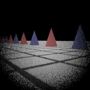
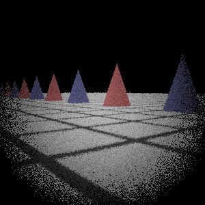
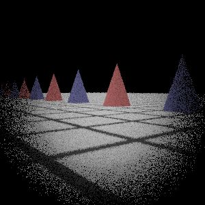
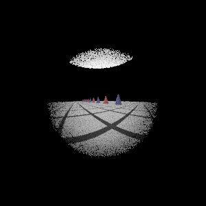
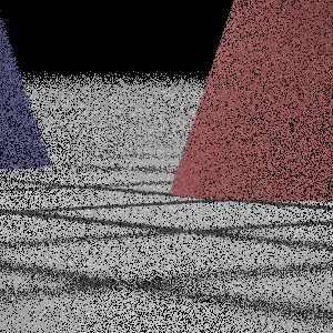
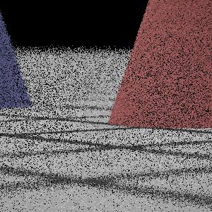
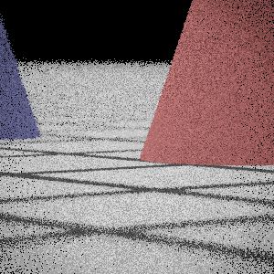
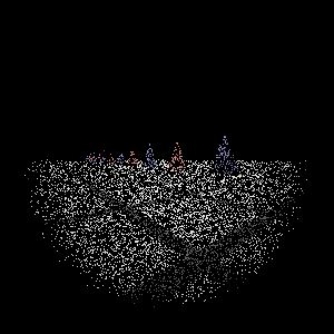
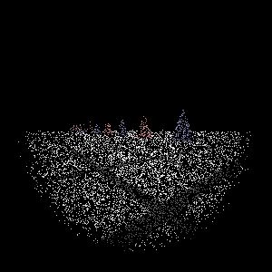
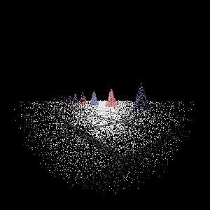
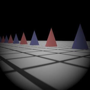
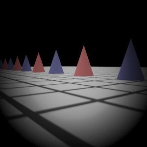
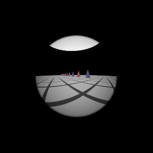
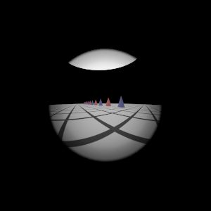
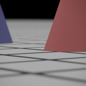
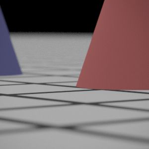
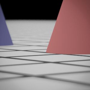
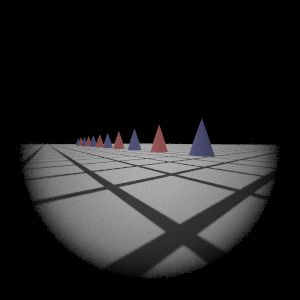
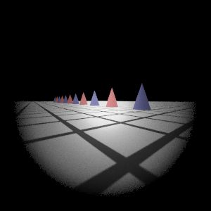
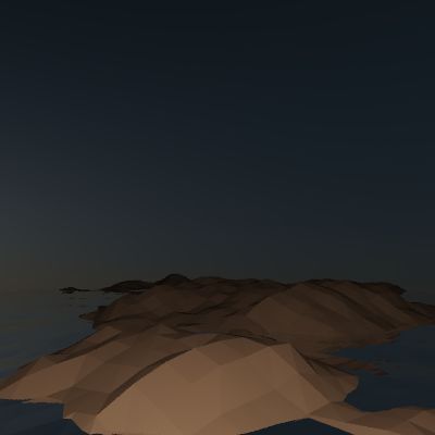
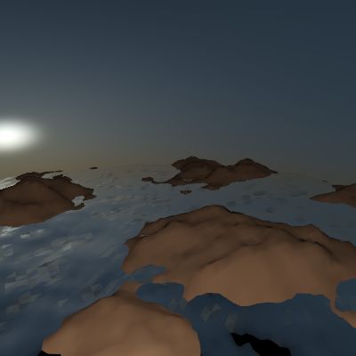
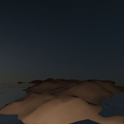
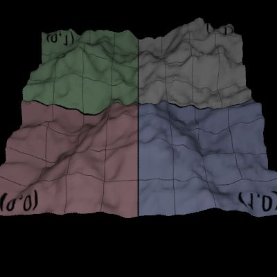
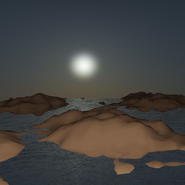
• pbrt.org scenes

Reference paper

Ray Specialized Contraction on Bounding Volume Hierarchies, Yan Gu Yong He Guy E. Blelloch

Median Cut Algorithm

根據論文 P. Debevec, A Median Cut Algorithm for Light Probe Sampling, SIGGRAPH 2006 Sketches and Applications. 中，預期要將 pbrt/lights/infinite.cpp 中的 class InfiniteAreaLight 用數個點光源取代 Infinite Area Light 的寫法，提升均勻取樣的效能，而 Median Cut Algorithm 在預處理非常快，根據用多少量的點光源將影響品質，若在品質不用太好的 rendering 環境下，這是一個不錯的降質提升速度的方案。

在 Median Cut Algorithm 取樣 64 equal-energy region 的速度在不同取樣個數差異比較

Env-Light.pbrt

Env-Light-new.pbrt

在 Median Cut Algorithm 不同數量 equal-energy region 在 256 samples 速度

Median Cut Algorithm equal-energy region

算法的步驟如下：

1. 將入射光場影像 (light probe image) 切成好幾個矩形區域，每一個區域將取用一個點光源代替。將入射光場影像轉換成灰階亮度 $Y$，如論文中所提及的方案 $Y = 0.2125 R + 0.7154 G + 0.0721 B$ 這類型的轉換。
2. 對於每一個區域將會根據最長維度切割成兩個子區域。切割成兩個子區域的亮度總和越接近越好。
3. 若切割區域數量不到目標的數量，則重複步驟 2。
4. 最後將每一個區域算出代表的點光源，並加總區域內的亮度和，隨後取樣根據亮度和作為取樣根據 (在 Spectrum MedianCutEnvironmentLight::Sample_L(const Point&, float, const LightSample&, float, Vector&, float*, VisibilityTester*) 中使用)，用每一個區域內部的 pixel 位置和亮度計算重心作為代表的點光源。

算法類似於 k-d Tree，但特別的是每次選擇區域維度最長的那一段進行切割，而不是像 k-d Tree 則是採用輪替維度進行。

Median Cut Algorithm 需要 $\mathcal{O}(HW)$ 時間 $\mathcal{O}(HW)$ 空間來預處理亮度資訊。若要切割成 $N$ 個區域，需要 $\mathcal{O}(\log N)$ 次迭代，每一次迭代增加兩倍區域數量。將一個區域切割時，針對維度最長的那一軸二分搜尋，二分搜尋計算其中一個區域的亮度和是否是整個區域亮度的一半，由於預處理完成的表格，可以在 $\mathcal{O}(1)$ 時間內計算任意平行兩軸的矩形內部元素總和。

維護 sumTable[i][j] 計算左上角 $(0, 0)$ 右下角 $(i, j)$ 的亮度和，計算任意平行兩軸矩形內部和只需要 $\mathcal{O}(1)$ 時間。

1
2
3
4
5
6
7

float getEnergy(float sumTable[], int width, int height) {
    float e = sumTable[VERT(ru, rv)];
    if (lu)	e -= sumTable[VERT(lu-1, rv)];
    if (lv)	e -= sumTable[VERT(ru, lv-1)];
    if (lu && lv)	e += sumTable[VERT(lu-1, lv-1)];
    return e;
}

另一種方案，可以從 pbrt 原生的 class MIPMap 取代上述寫法，MIPMap 的寫法採用分層式的架構，每一層將原圖長寬各縮小一半。計算某矩形元素總和時，藉由兩層的總和估計進行內插。理論上，這種寫法雖然不夠精準，但提供很好的快取優勢。

重心計算

Centroid Formula 1

一般重心計算採用以下公式：

經由 Median-Cut Algorithm 在 Texmap 1 運行後，代表的點光源明顯地偏離亮區，因此為了讓代表的點光源更靠近亮區，我們將其重心公式修改成 Centroid Formula 2。

Centroid Formula 1

若以 $\mathit{Energy} \propto L^2_{(x, y)}$，能量與亮度二次成正比，則計算出的重心會更靠近亮區。

比較結果如下：

由於 CSS 問題，詳細內容請到 http://morris821028.github.io/hw-rendering/homework3/submission/index.html 觀看。

Ray Sphere Intersection

計算射線和球體的交點，可以參照 /pbrt-v2/shapes/sphere.cpp 中 bool Shpere::Intersect() 的算法。

假設球體圓心座標 $O$，射線單位向量 $I$ 的起點座標 $C$，且最近目標交點座標 $P$，原半徑 $\mathrm{radius}$。射線走單位時間 $t$ 會到達球面上。

• $\overrightarrow{OC} + \overrightarrow{I} \times t = \overrightarrow{OP}$
• $|\overrightarrow{OP}| = \text{radius}$
• $|\overrightarrow{OC} + \overrightarrow{I} \times t| = |\overrightarrow{OP}|$
• $|\overrightarrow{I}|^2 t^2 + 2 \; (\overrightarrow{OC} \cdot \overrightarrow{I}) \; t + |\overrightarrow{OC}|^2 - \text{radius}^2 = 0$

解一元二次方程式之後可以得到 $t$ 得值，並得到交點座標 $P$。

Snell’s Law

根據物理法則斯乃爾定律計算折射的方向向量，課程中提供三種做法。

變數解釋：入射介面材質 $\eta_1$，折射介面材質 $\eta_2$，入射單位向量 $\overrightarrow{I}$，交點面法向量 $\overrightarrow{N}$，折射方向向量 $\overrightarrow{T}$

特別小心 ray->d = Normalize(ray->d) 的處理，Heckbert’s Method 計算維持在單位圓上，故不用做最後的正規化計算。

Whitted’s Method

Heckbert’s Method

Other Method

其中以 Heckbert’s Method 消耗最少計算數。如果除法速度快於乘法，則使用 Other Method，原則上很少有機器運算除法比乘法快。

RasterToCamera

這部分處理後得到 Transform RasterToCamera。若計算錯誤，會造成一片黑或者圖片顯示的大小問題。座標轉換處理細節可以參考實際的例子，如下圖所示：

• Raster-To-NDC 轉換矩陣 $A=\text{Scale}(scale, scale, 1)$，進行縮放。
• NDC-To-Camera 轉換矩陣 $B=\text{Translate}(Vector(0, 0, filedistance)) \times \text{Translate}(Vector(X, -Y, 0))$，進行位移。
• 最後得到 RasterToCamera 轉換矩陣 $C= B \times A \times \text{Scale}(-1, 1, 1)$，最後將 x 軸顛倒以符合成像問題。

Ray Weight

作業要求經過 float GenerateRay() 回傳 $\mathrm{weight} = \frac{\cos^4 \theta'}{Z^2}$，這麼設置會過暗，根據論文 A Realistic Camera Model for Computer Graphics 中寫道

If the exit pupil subtends a small solid angle from $x'$, $\theta'$ can be assumed to be constant and equal the angle between $x'$ and the center of the disk. This allows us to simplify
$E(x') = \int_{x'' \in D} L(x'', x') \frac{\cos \theta' \cos \theta''}{\| x'' - x'\|} dA''$<span>$to:$</span><!-- Has MathJax -->$E(x’) = L \frac{A}{Z^2} \cos^4 \theta’$
where $Z$ is the axial distance from the film plane to the dist and $A$ is the area of the disk.

因此需要額外乘上常數 $A$，其中 $A$ 是最裡層的透鏡面積，因為我們是根據最裡層的透鏡面做均勻取樣，得到 $A = \mathit{backLens.radius}^2 \pi$。

Sampling

單位圓均勻取樣方法有以下兩種，而非均勻取樣的寫法可參照 Sample 3 (錯誤的做法參照) 出來的效果看出。

Sampling 1

採用內建函數 CencentricSampleDisk()，採用 A Low Distortion Map Between Disk and Square 論文中提到的方案，將一個正方形壓縮到一個圓形中。參照作法如下圖所示

其中給定 $a, b$ 均勻分布 $[0, 1]$，則得到 $r = a, \; \phi = \frac{\pi}{4} \frac{b}{a}$，最後計算得到座標 $x = r \cos \phi, \; y = r \sin \phi$。

Sampling 2

採用教科書上提供，其中給定 $a, b$ 均勻分布 $[0, 1]$，令 $r = \sqrt{a}, \; \phi = 2 \pi b$，最後計算得到座標 $x = r \cos \phi, \; y = r \sin \phi$。

Sampling 3

分布 $[0, 1]$，令 $r = a, \; \phi = 2 \pi b$，最後計算得到座標 $x = r \cos \phi, \; y = r \sin \phi$。這種寫法在相同半徑下，角度均勻分布，不同半徑下的周長與 $r$ 成正比，導致不同半徑的取樣點不均勻，越靠近中心點取樣越密集，意即容易造成中心點看起來較亮。

Reference

• PBRT学习笔记：在单位圆内部均匀采样 -
  codeboycjy的专栏

Final Images Rendered Compare 4 samples

Gauss Lens

My Implementation (Sampling 1)

My Implementation (Sampling 2)

My Implementation (Sampling 3)

Fisheye Lens

My Implementation (Sampling 1)

My Implementation (Sampling 2)

My Implementation (Sampling 3)

Telephoto Lens

My Implementation (Sampling 1)

My Implementation (Sampling 2)

My Implementation (Sampling 3)

Wide-Angle Lens

My Implementation (Sampling 1)

My Implementation (Sampling 2)

My Implementation (Sampling 3)

Final Images Rendered Compare 512 samples

Gauss Lens

Reference

My Implementation (Sampling 1)

My Implementation (Sampling 2)

My Implementation (Sampling 3)

Fisheye Lens

Reference

My Implementation (Sampling 1)

My Implementation (Sampling 2)

My Implementation (Sampling 3)

Telephoto Lens

Reference

My Implementation (Sampling 1)

My Implementation (Sampling 2)

My Implementation (Sampling 3)

Wide-Angle Lens

Reference

My Implementation (Sampling 1)

My Implementation (Sampling 2)

My Implementation (Sampling 3)

前情提要 pbrt

一套數位影像生成軟體，盡可能以物理性質為基底打造的，目前已經到了 pbrt-v3。pbrt 主要的工作在於 modeling 後，可以在場景內放置以幾何描述的物體、光源、拍攝曝光 … 等設定，藉由模擬光線走訪得到呈現在螢幕上每一個 pixel 的顏色。

目標工作

Height Field 是一個高度場，測資中以山脈構造為主，等間隔取樣每一平面上的每一點高度的場景，當間隔越小越接近真實場景。原生寫法是將點放置在三維空間，轉換成一堆三角網格，將其丟入 KD-tree 或者是 BVH 等加速結構，加快光線模擬找交點 (三維空間中，一射線和一多面體的交點) 的效能。而現在挑戰用 3D-DDA 的方式進行交點查找。

實作採用 3D-DDA 算法降至 2D Grid 上進行交點測試。Uniform Grid 將會切割成 $N \times M$ 的格子，在 2D 平面上，先找到 ray 進入的格子點，接著使用增量算法找到下一個格子，算法只測試投影到 x-y 平面上時，在 ray 鄰近的格子點做交點測試，時間複雜度 $O(\sqrt{N \times M})$，與預設的其他算法所需要的 traversal 複雜度差不多。

原本預設的 Height Field 拆成好幾個 Triangle，做法類似 Triangle Mesh，接著將這幾個 Triangle 利用 BVH 或者是 KD-tree 的架構進行，原本的做法會考慮三個維度，使用投影的方式只考慮兩個維度下的情況，接著再針對有相交的格子測試，最後才進行 3D Triangle 是否與 ray 相交。

實作 Height Field 時，考慮快取和再計算之間的好壞，則有兩種方法

1. 預先將預處理每個 3D Triangle 座標 (消耗空間)
2. 需要時，再創建 Triangle 出來測試 (消耗時間)

由於要找 ray 碰度到 uniform grid 的第一個格子，需要預處理 Height Field Bound Box，計算 Bound Box 需要 $O(N \times M)$，若不預處理會造成 3D-DDA 與暴力法 $O(N \times M)$ 無異。

若對 Height Field 進行 2D-DDA 好處在於一定是數個三角形構成，因此不用等到 ray.maxT 小於下一格交點的 NextCrossingT[stepAxis] 才能結束，一與三角形有交點就可以離開，因為每一格之間都有獨立性。

實作與測試細節

測試環境

一開始為了熟悉 pbrt 架構環境只實作求出交點的函數，

1
2
3
4

bool Heightfield2::Intersect(const Ray &r, float *tHit, float *rayEpsilon,
        DifferentialGeometry *dg) const {
    // 3D DDA
}

而直接忽略單純詢問交點是否存在，這會導致畫面一片黑，因為每打到一個交點會嘗試從物體表面的交點連到點光源。若下述函數恆真，則不存在光源到交點的路徑，因此產出來的圖片是一片黑。

1
2
3

bool Heightfield2::IntersectP(const Ray &r) const {
    return true;
}

紋理模糊

找出紋理的兩個參數 $(u, v)$ 時，從 trianglemesh.cpp 複製過來的 class Triangle 其 bool Triangle::Intersect() 函數得到的 $u, v$ 都是相對於三角形的 $0 \le u, v \le 1$ (直接 rendering 會看起來很多小格子點)，因此得到相對的 $u, v$ 和交點 $p_{hit}$ (Object coordinate)，則把 $p_{hit}$ 再次投影到 x-y 平面上，由於 height field 在 x-y 平面上長寬都是 1，投影到平面後得到 $p_{projection}$，對於整個 height field $u = p_{projection}.x, \; v = p_{projection}.y$。

若測試 texture.pbrt 時，發生過模糊情況，其主要原因在於過多次座標轉換，如 Object -> World -> Object -> World，求出來的 $u, v$ 誤差就會放大。

將 height field 存成好幾個 triangle 可以像 class TriangleMesh 利用 index 標籤來壓縮記憶體，但實作為方便仍然每一個三角形都有實體的 Point，儲存三角形每一個點座標採用 object coordinate，先把 $ray$ 從 WorldToObject 得到 $ray'$，得到的交點 $p_{hit}$ 再進行 ObjectToWorld，如此一來模糊情況就會消失。

Phong 圓滑化

Phong interpolation 方法在三角形上面操作時，需要得知三個頂點的法向量，給予 height field 的資訊，並不曉得每一個頂點的法向量為何。得到每一個頂點的法向量，採用預先處理所有頂點的法向量並儲存起來，因為不斷地正規化是很耗時間的 (float sqrt(float x) 儘管採用 fast inverse square root 算法，也要極力避免多餘的運算)。

再計算頂點法向量時，根據影像處理中常用的一次差分 (differentiation) 遮罩

Case 1 邊緣

Case 2 非邊緣

上圖矩陣的中心座標為 $(x, y)$，將相鄰座標的高度值 $z$ 相減得到兩個方向的向量 $N_x, \; N_y$，外積得到座標 $(x, y)$ 的法向量 $N_{x, y} = \mathrm{Cross}(N_x, N_y)$。

從另一個角度來看，將 height field 三角化後，每一個頂點原則上有 6 個鄰居，可以對每一個鄰居進行差分，接著順時針或者逆時針將兩兩相臨的向量外積，得到 6 個法向量平均後得到 $N_{x, y}$，這做法看起來比上述的差分來得穩定，但初始化消耗的時間會比較長，且撰寫的外積順序不對容易造成零向量的正規化錯誤。

Final Images Rendered with my implementation of heightfield.cpp

hftest.pbrt (without Phong interpolation) Timings: Original: 0.125 seconds My implementation: 0.130 seconds (104% original)	landsea-0.pbrt (without Phong interpolation) Timings: Original: 0.815 seconds My implementation: 1.050 seconds (128% original)
landsea-1.pbrt (without Phong interpolation) Timings: Original: 0.850 seconds My implementation: 1.020 seconds (120% original)	landsea-2.pbrt (without Phong interpolation) Timings: Original: 0.780 seconds My implementation: 0.870 seconds (115% original)
texture.pbrt (without Phong interpolation) Timings: Original: 0.450 seconds My implementation: 0.520 seconds (120% original)
landsea-big.pbrt (without Phong interpolation) Timings: Original: 6.200 seconds My implementation: 2.200 seconds (35% original)

Final Images Rendered with my implementation of heightfield.cpp

hftest.pbrt (with Phong interpolation) Timings: My implementation: 0.135 seconds	landsea-0.pbrt (with Phong interpolation) Timings: My implementation: 1.100 seconds
landsea-1.pbrt (with Phong interpolation) Timings: My implementation: 1.050 seconds	landsea-2.pbrt (with Phong interpolation) Timings: My implementation: 0.900 seconds
texture.pbrt (with Phong interpolation) Timings: My implementation: 0.530 seconds
landsea-big.pbrt (with Phong interpolation) Timings: My implementation: 2.300 seconds